EarthDefine Clutter3D: Technical Specification
Oct 7, 2026
How EarthDefine produces and delivers Clutter3D for RF planning: the source data, the 20-class classification scheme, density and overlap rules, terrain and feature heights, accuracy assessment, and delivery formats.
It'll only take a few seconds.
Generated from this page, last revised 8 October 2026. The link always serves the current version.
See also: Clutter3D sample data
1. What is Clutter3D?
EarthDefine Clutter3D combines a 20-class clutter classification with above-ground feature heights, bare-earth terrain elevation, building footprints, and aerial imagery.
Clutter classification, feature height, and terrain elevation describe different properties of the same location:
- Clutter classification identifies the surface or obstruction category.
- Feature height describes the vertical extent above the underlying ground.
- Terrain elevation describes the ground elevation relative to sea level.
These layers support RF propagation modeling, coverage analysis, and wireless network planning. Classification and elevation rasters are delivered at 1-meter resolution. Buildings are delivered as vectors; accompanying imagery retains its source resolution.
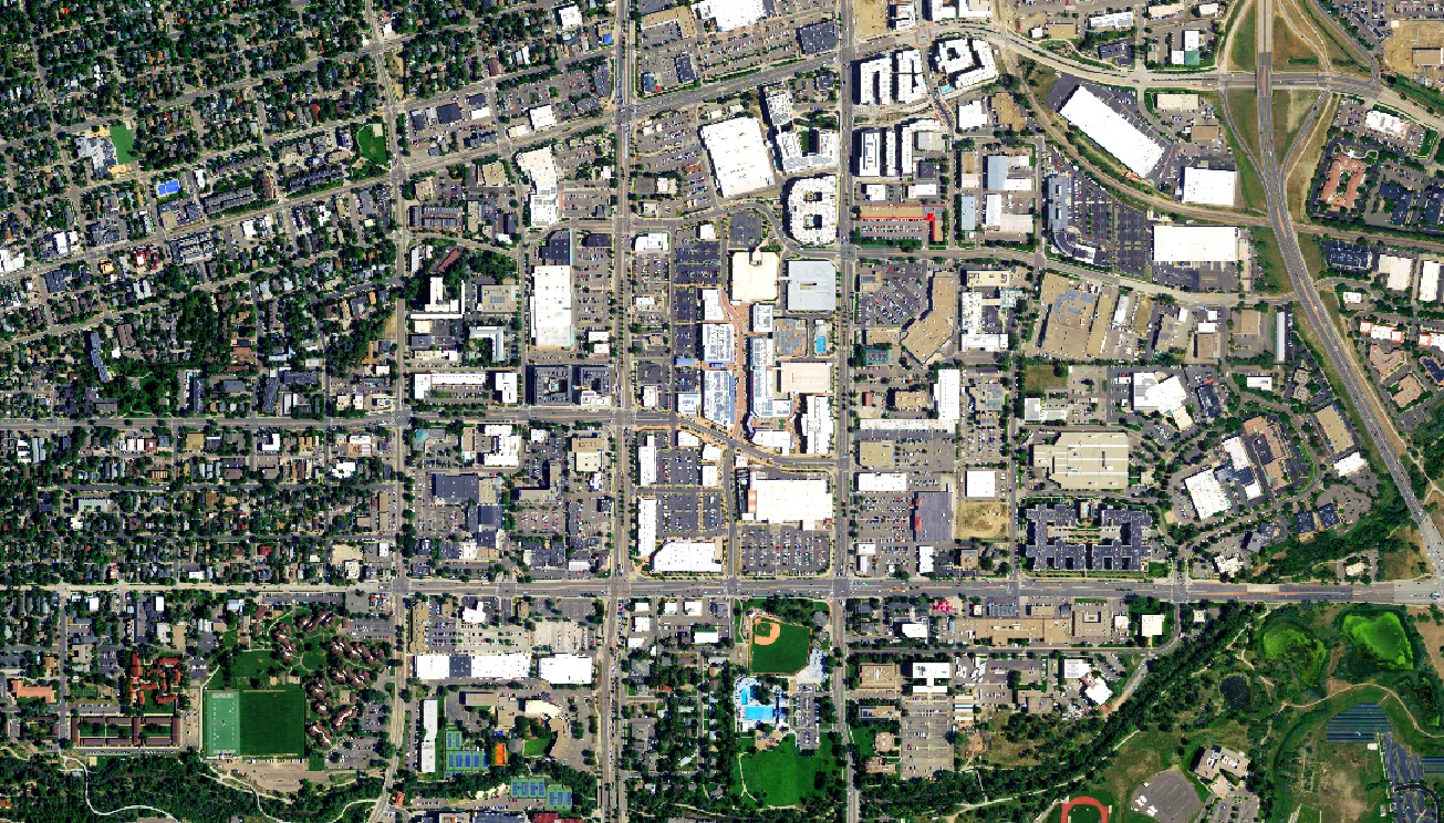
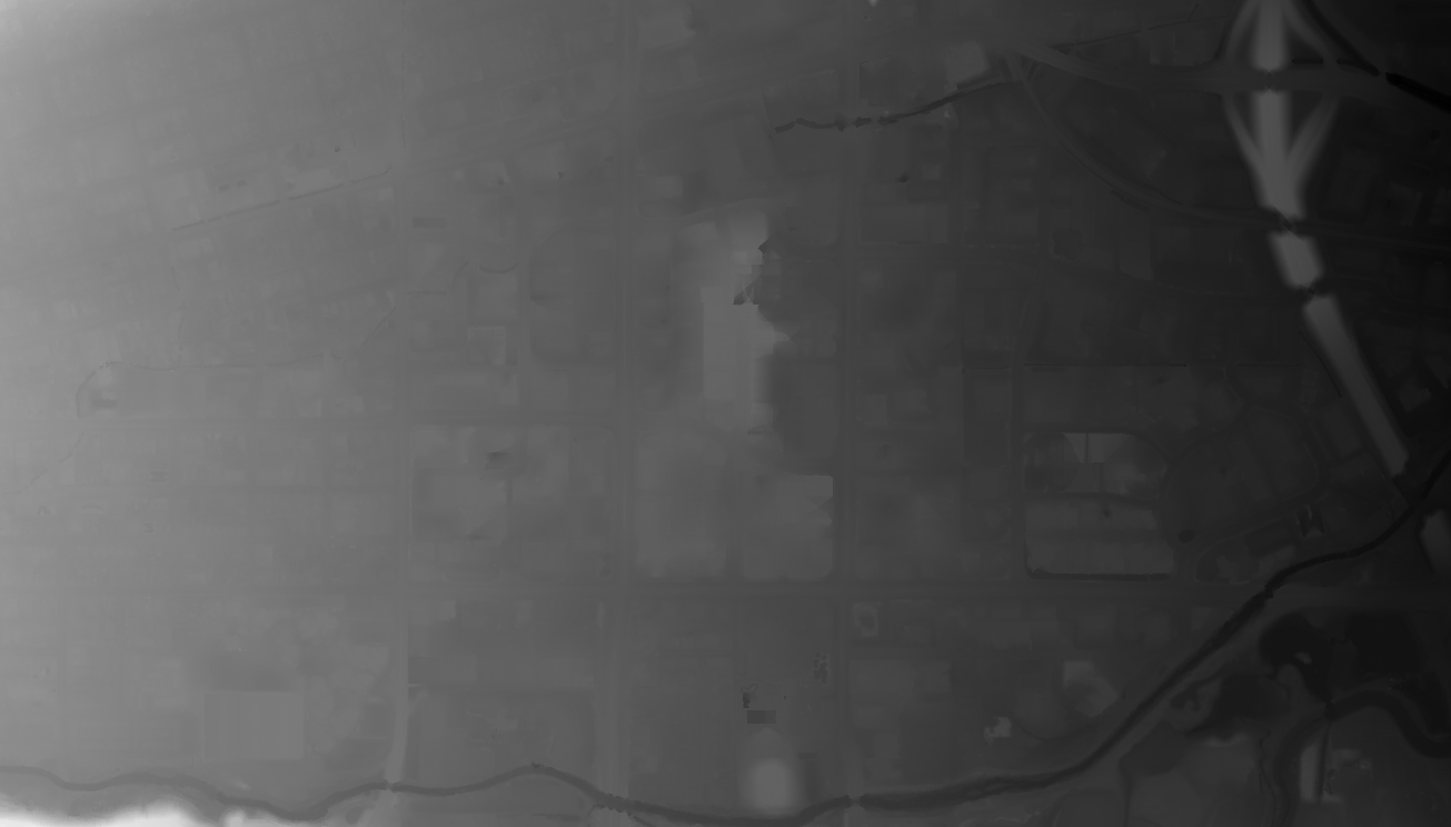
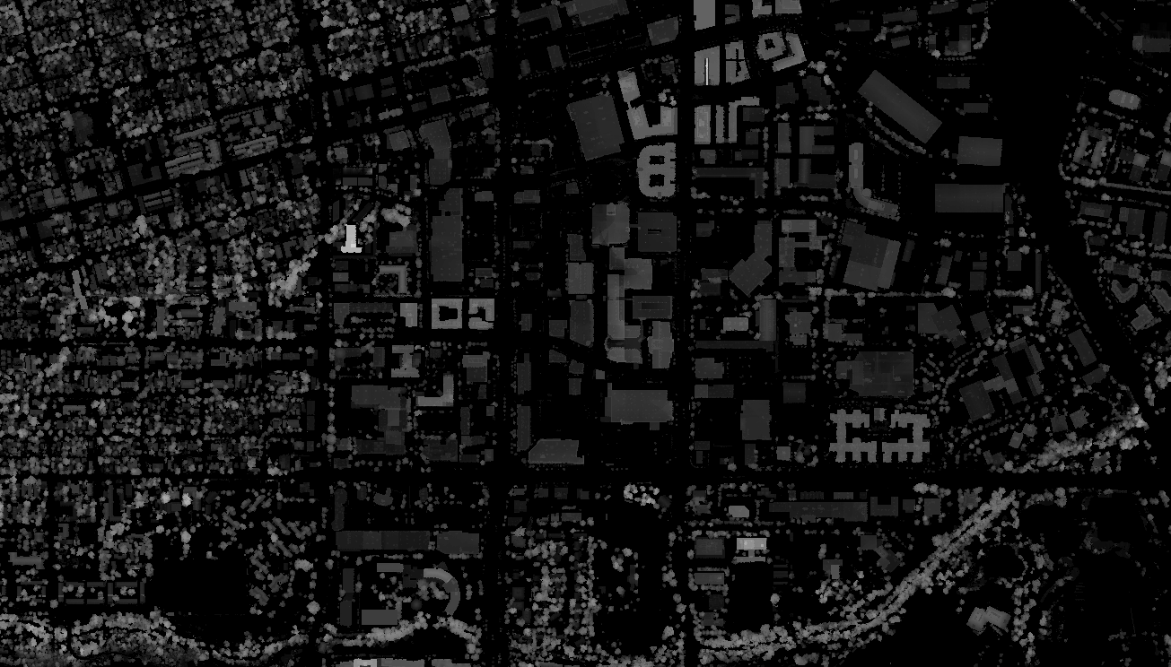
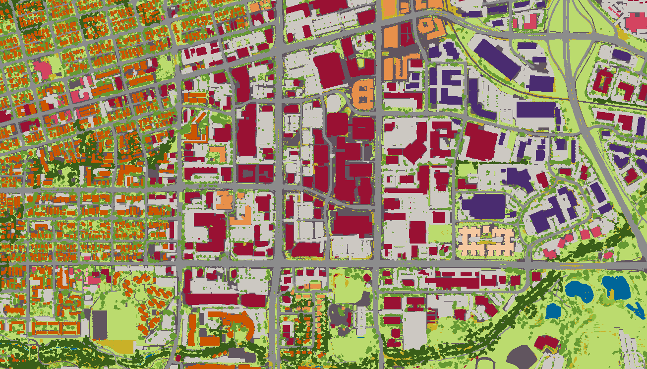
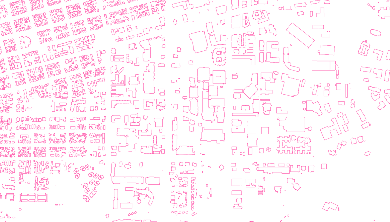
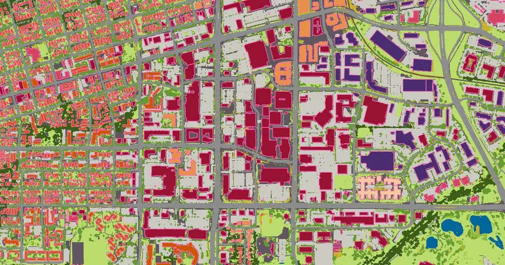
Figure 1. Clutter3D for Boulder, CO, over the aerial imagery. Switch the layers to compare the classification with terrain, feature heights and building footprints.
2. Where is it available?
Clutter3D is available across the contiguous United States, Hawaii, Puerto Rico, and the US Virgin Islands.
Deliveries are scoped to an area of interest. Classification and height production draw on the available sources for that geography. Heights may be LiDAR-derived, interpolated, or estimated, so complete geographic coverage does not imply a direct LiDAR measurement at every location.
EarthDefine can help customers identify where heights are LiDAR-derived and where estimates are used.
Figure 2. Clutter3D availability: the contiguous United States, Hawaii, Puerto Rico, and the US Virgin Islands.
3. Where does the data come from, and how is it produced?
Clutter3D combines EarthDefine Land Cover, Building Footprints, LiDAR-derived elevation, parcel land-use information, transportation data, parking polygons, and proprietary models and algorithms.
Land Cover and imagery
The underlying Land Cover pipeline classifies USDA NAIP four-band color-infrared aerial imagery, typically acquired at 30cm to 60cm resolution. Class-specific convolutional neural networks identify surface-cover features. LiDAR-derived elevation and ancillary planimetric information supplement the imagery where they improve classification.
Training data combines manual photointerpretation, stratified sampling, and existing labeled Land Cover archives. Model selection uses Intersection over Union against held-out validation and test sets.
The base outputs are merged and post-processed, including gap filling and filtering of isolated pixel artifacts.
Buildings and land use
Building geometry comes from EarthDefine Building Footprints. Available parcel land-use structure codes are mapped to residential, commercial, or industrial use.
Where those codes are unavailable, a machine-learning classifier predicts building use from building geometry, height, parking, and neighborhood context. Connected structures share a use prediction across their component polygons.
Transportation and parking
Road surfaces can come directly from a dedicated Land Cover road class. Where this is unavailable, transportation centerlines are expanded into road-surface masks according to road category.
Railway data provides rail corridors. Airport tarmac areas are delineated during review; within those areas, applicable impervious and road surfaces become the airport class. Parking polygons supply the parking class.
Assembly
Source layers are prepared in a common processing coordinate system and grid. Vegetation and building density are calculated, class-precedence rules resolve overlaps, heights are processed, and outputs are masked to the requested boundary.
4. What are the 20 clutter classes?
| Code | Color | Class | Interpretation |
|---|---|---|---|
| 10 | Water | Open water | |
| 20 | Bare Earth | Bare ground and the base classification | |
| 31 | Ground-level Vegetation | Ground-level vegetated surfaces | |
| 32 | Low Vegetation | Low vegetation distinguished using Land Cover and height | |
| 33 | Tree, Low Density | Tree canopy in smaller connected patches | |
| 34 | Tree, High Density | Tree canopy in larger connected patches | |
| 41 | Residential, Low Density | Residential buildings below the medium-density threshold | |
| 42 | Residential, Medium Density | Residential buildings between the medium and high thresholds | |
| 43 | Residential, High Density | Residential buildings at or above the high threshold | |
| 51 | Commercial, Low Density | Commercial buildings below the medium-density threshold | |
| 52 | Commercial, Medium Density | Commercial buildings between the medium and high thresholds | |
| 53 | Commercial, High Density | Commercial buildings at or above the high threshold | |
| 61 | Industrial, Low Density | Industrial buildings below the medium-density threshold | |
| 62 | Industrial, Medium Density | Industrial buildings between the medium and high thresholds | |
| 63 | Industrial, High Density | Industrial buildings at or above the high threshold | |
| 71 | Parking | Parking areas identified from parking polygons | |
| 72 | Roads | Road surfaces | |
| 73 | Railways | Rail corridors | |
| 74 | Airports | Delineated airport tarmac surfaces | |
| 75 | Other Impervious | Remaining impervious surfaces |
Building use is broader than a simple visual interpretation of the roof. Commercial includes office, retail, institutional, transportation-terminal, and military structures. Industrial includes manufacturing, warehousing, utility, and agricultural structures.
10 Water
20 Bare Earth
31 Ground-level Vegetation
32 Low Vegetation
33 Tree, Low Density
34 Tree, High Density
41 Residential, Low Density
42 Residential, Medium Density
43 Residential, High Density
51 Commercial, Low Density
52 Commercial, Medium Density
53 Commercial, High Density
61 Industrial, Low Density
62 Industrial, Medium Density
63 Industrial, High Density
71 Parking
72 Roads
73 Railways
74 Airports
75 Other Impervious
Figure 3. Aerial imagery typical of each clutter class, labelled with its code and map color.
5. How are density categories defined?
Building density
Building density is calculated separately for residential, commercial, and industrial structures.
For each structure, EarthDefine identifies neighboring structures of the same use type within 500 meters of its centroid. Their combined footprint area is divided by the area of the 500-meter-radius circle.
This measures same-type building footprint coverage. It does not measure population density, parcel count, or total developed land.
| Building use | Low density | Medium density | High density |
|---|---|---|---|
| Residential | Below 2% | 2% to below 8% | 8% or greater |
| Commercial | Below 2% | 2% to below 5% | 5% or greater |
| Industrial | Below 2% | 2% to below 5% | 5% or greater |
These are the standard processing defaults and can be adjusted for a project.
Component polygons belonging to the same contiguous structure are combined before density calculation. Each structure receives an area-weighted centroid and summed footprint area, allowing its component polygons to receive a consistent density category.
The calculation includes buildings within a 500-meter buffer around the area of interest, reducing boundary effects. A second density measure at 150 meters is included in the building attributes for finer local analysis; the 500-meter measure determines the standard density category.
Tree density
Tree density uses the area of connected canopy patches. Tree pixels touching along an edge or corner belong to the same patch.
- Patches smaller than 2,500 m² receive Tree, Low Density.
- Patches of 2,500 m² or larger receive Tree, High Density.
This is a canopy-patch classification, rather than a count of individual trees or a measure of stems per hectare.
Vegetation height
Vegetation classification combines the underlying Land Cover category with nDSM height. Standard height breaks are 0.5 meters and 3 meters, with different treatment according to the input vegetation class. Pixels already identified as trees, including trees over impervious surfaces, enter the tree-density calculation.
These clutter rules are distinct from the approximately 10-foot tree/shrub boundary used to develop training labels for the underlying Land Cover product.
Figure 4. Building density categories: the same neighborhood classified at low, medium and high density for one building use.
6. Which class takes priority where features overlap?
Clutter3D assigns one final class to each raster cell. Layers are combined in a defined order, with later layers taking priority over earlier ones.
From highest to lowest priority:
- Buildings
- Vegetation
- Parking
- Other impervious surfaces
- Transportation surfaces
- Water and the bare-earth base
Within transportation processing, roads are applied before railways and airports; airports can replace roads within delineated tarmac areas.
Worked examples
Tree canopy over a road or parking lot. The vegetation class takes priority over the underlying transportation or parking surface.
Tree canopy overlapping a building footprint. The building class takes priority over vegetation.
Airport containing buildings and vegetation. Airport classification applies to eligible road and impervious surfaces within the delineated area. Buildings and vegetation retain their higher-priority classes.
Driveway or sidewalk outside other mapped features. Remaining impervious pixels receive Other Impervious.
The classification and height layers remain separate. Class precedence determines the final category; it does not by itself establish how every height value is assigned.
(a)
(b)
Figure 5. Class precedence where features overlap: (a) the imagery, (b) the final class assigned to each cell.
7. How are terrain and feature heights represented?
The DEM represents bare-earth terrain elevation in meters above mean sea level. The heights raster represents feature height in meters above ground level.
For corresponding cells with compatible references:
Surface elevation = terrain elevation + above-ground feature height
LiDAR processing
Height processing starts from LiDAR-derived first-return nDSM data where available. Gaps are interpolated within a configured distance, and interpolated values are retained within the applicable feature mask.
A local spike filter reduces isolated elevation artifacts. Standard processing uses a 3 × 3 kernel and a 100-meter spike threshold.
Buildings absent from the height data
Building footprints with mean nDSM height below 2 meters are treated as candidates for replacement height estimates. This is a processing rule for inadequate height representation; it is not independent proof of a building's construction date.
Replacement heights follow this order:
- The 75th percentile of heights among same-type buildings within 250 meters.
- The 75th percentile among any-type buildings within 250 meters, if suitable same-type neighbors are unavailable.
- A fixed building-type fallback if suitable neighbors are unavailable.
| Building use | Default fallback height |
|---|---|
| Residential | 8 meters |
| Commercial | 12 meters |
| Industrial | 10 meters |
These values are estimates and are configurable.
Trees with inadequate height data
Tree pixels with height below 2 meters can receive nearby valid tree heights through distance-limited interpolation. The interpolation draws from tree-classified pixels with valid height values, rather than from buildings or bare ground.
Remaining tree pixels receive a configurable fallback, defaulting to 4 meters. An optional tree-height adjustment can also be applied; the documented example runs use no additional adjustment.
Building height attributes
The building vector's AGL field represents maximum building height above ground, rather than mean roof height. Where a measured height is unavailable, the documented estimation hierarchy applies.
AMSL represents rooftop elevation: terrain elevation at the building location plus AGL.
(a) DEM
(b) Feature height
Figure 6. The two elevation layers for Boulder, CO: (a) DEM, bare-earth terrain in meters above mean sea level; (b) feature height in meters above ground level.
8. How is accuracy measured and quality verified?
Underlying Land Cover accuracy
EarthDefine randomly generates 1,000–5,000 assessment points within each state boundary, depending on the state's size.
A team member reviews each point against NAIP imagery and assigns its reference class. Each reference assignment is compared with the Land Cover raster prediction, producing a confusion matrix of predicted versus reference classifications.
EarthDefine's national Land Cover product targets greater than 95% overall accuracy per state using this method. Client Land Cover products are delivered at 95% overall accuracy or higher, and accuracy assessments are usually included in standard Land Cover deliverables.
This assessment measures the underlying Land Cover classification. It does not independently validate every building-use or density category in the final 20-class clutter output.
Height accuracy
For LiDAR-derived building heights, EarthDefine follows the source-dependent approach documented in the Building Footprints 3D technical specification. No single product-wide height-accuracy figure is published; the underlying LiDAR collection's vertical specification is available for an area of interest.
Neighbor-based estimates, interpolated heights, and fixed fallback values should be interpreted separately from direct LiDAR-derived measurements.
A 1-meter raster resolution describes pixel size. It does not establish 1-meter positional accuracy or a particular vertical-accuracy value.
Production review
The underlying Land Cover pipeline includes automated checks, regular-grid human review, and correction against source imagery.
The documented clutter workflow also supports review and correction of predicted building-use assignments before rasterization. Edited assignments are checked against the permitted residential, commercial, and industrial categories.
These are production quality controls, distinct from statistical accuracy assessments.
9. What is delivered?
| Component | Standard representation | Units or values |
|---|---|---|
| Clutter classification | Single-band, 8-bit GeoTIFF; LZW compressed | The 20 class codes |
| Feature heights | Float32 raster | Meters above ground |
| DEM | Float32 raster | Meters above mean sea level |
| Building footprints | Polygon shapefile | Height, use, density, and area attributes |
| Aerial imagery | GeoTIFF | RGB imagery |
| Area-of-interest boundary | Vector boundary | Delivery extent |
| QGIS project | .qgs | Prepared layer display |
| README | Text | Product and field reference |
Clutter, heights, and DEM rasters are delivered at 1-meter resolution. Output uses WGS84 UTM, with the zone selected from the area of interest. Exact coordinate-system details are recorded in the delivered files.
The clutter raster includes a Raster Attribute Table in an .aux.xml sidecar, mapping codes to class labels, categories, and colors. The QGIS project uses relative layer paths and includes prepared symbology.
Building attribute dictionary
7 fields
| Field | Type | Description |
|---|---|---|
AGL
|
Real | Maximum building height above ground, in meters; measured or estimated |
AMSL
|
Real | Rooftop elevation above mean sea level, in meters |
Class
|
Text | Residential, Commercial, or Industrial |
SubClass
|
Text | Low, medium, or high density |
Area_SqMts
|
Real | Building footprint area in square meters |
den_500m
|
Real | Same-type footprint coverage fraction within 500 meters |
den_150m
|
Real | Same-type footprint coverage fraction within 150 meters |
Zero values and the delivery boundary
The documented workflow masks values outside the area of interest to zero. The clutter raster uses zero outside the boundary.
In the heights raster, zero is also a valid above-ground height, and the documented output has no separate NoData value. Customers should therefore use the delivered boundary when distinguishing valid zero-height locations from areas outside the delivery.
Large deliveries may be tiled. GeoTIFF is the standard raster format; alternate raster formats and project-specific configurations can be arranged.
Figure 7. The delivered QGIS project, with the prepared layer symbology.
10. How current is the data?
Land Cover conditions correspond to the acquisition date of the source imagery. Heights and transportation information may derive from sources acquired at different times.
New imagery can reveal buildings or vegetation that are absent from older LiDAR. The height-estimation and interpolation rules described above address these cases without treating the resulting heights as direct measurements.
Deliveries include source imagery metadata. Customers can consult EarthDefine about source availability and height provenance for their area of interest.
11. How is it delivered and licensed?
Deliveries are scoped to the customer's area of interest and planning requirements. The standard package brings classification, feature heights, terrain, buildings, imagery, and visualization files together for evaluation and integration.
Commercial pricing and usage terms are established for the requested geography and use case.
Custom density thresholds, height assumptions, raster formats, and other processing settings are available where a project requires a different configuration. Customers can evaluate a sample in their planning environment before defining a production delivery.
It'll only take a few seconds.
Generated from this page, last revised 8 October 2026. The link always serves the current version.
Related products
Clutter3D
Telecom's most precise RF clutter dataset. Signal-aware classes, per-pixel LiDAR heights, nationwide at 1m resolution.
Learn more